Implementing Trajectories in Games

This project will analyse some different methods of constructing trajectories from player input. It also features some code written to keep the endpoint of a trajectory stationary whilst one component of the trajectory in 3-dimensional space is altered, as well as a discussion of the mathematics behind this approach. The trajectories have been implemented in 2D using the Godot Engine (see this project for more details) and in 3D using Unreal Engine (see this project for more details).

Launch Angles vs Velocity Vectors

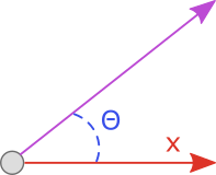
Generally, there are two main ways to represent trajectories in 3D space - as a length \(l\) and angles from the origin \((\theta_y,\theta_z)\) or as a 3-dimensional vector \((x,y,z)\). Within game development, it is more natural to use the vector representation - the majority of physics engines all use this representation to calculate forces, velocities, impulses and more. However, it turns out that the representations are equivalent anyway, and a conversion exists between them. The example below highlights this for a simple case in 2D - we can convert the trajectory represented by length \(l\) and angle \(\theta_y\) to the same trajectory represented by the vector \((x,y)\)

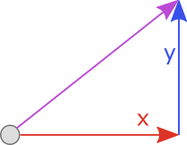Angle representation	Vector Representation

Some simple vector geometry provides the following conversions from \((x,y)\) to \(l\) and \(\theta_y\): $$l = |(x,y)| = \sqrt{(x^2+y^2)}$$ $$\theta_y = \tan^{-1}(\frac{y}{x})$$ The reverse conversion is given by the equations: $$x = l\cos(\theta_y)$$ $$y = l\sin(\theta_y)$$ Hence, since the conversion between trajectory representations is linear in its time complexity, the choice is largely irrelevant. As mentioned before, this report will choose to use the 3-dimensional vector \((x,y,z)\) as this is the preffered choice in game engines.

Constructing Trajectories from Input

In this section, we will consider a few methods of constructing a trajectory from player input. The difference between each method is essentially how many sources of input to take. With more sources of input, the player generally has a higher degree of precision. However, this does come at the cost of making the control scheme more complex and potentially lengthening the aiming process. This tradeoff should be carefully considered with regards to the design intent of the game being developed.

Single Input (2D)

Calculating a trajectory ((x,y)) with a single input is possible in 2D. In my 2D Golf project, I use the user’s mouse position to populate the trajectory vector ((x,y)) with the following calculation:

Where (mouse_x) is the x-component of the mouse position and (target_x) is the x-component of the projectile to be launched. This method is quick and allows the user to generate any possible trajectory with only a single input (mouse movement).

Generating a trajectory with a single input

The code block below demonstrates this technique. The line of particular relevance is the funcion call to apply_central_impulse(). Note that the trajectory vector passed as an argument is first clamped to a predetermined value (max_impulse) before being multiplied by the scalar shot_power. This imposes a limit on the power that the user can generate.

func attempt_shot(click_position):
	if ready and can_shoot:
		apply_central_impulse((click_position-position).clamped(max_impulse)*shot_power)
		ready = false
		tracking = false
		shot_tracer.clear_trace()
		friction_timer.start()
		if player_man.shot_taken():
			can_shoot = true
		else:
			can_shoot = false

Double Input (2D)

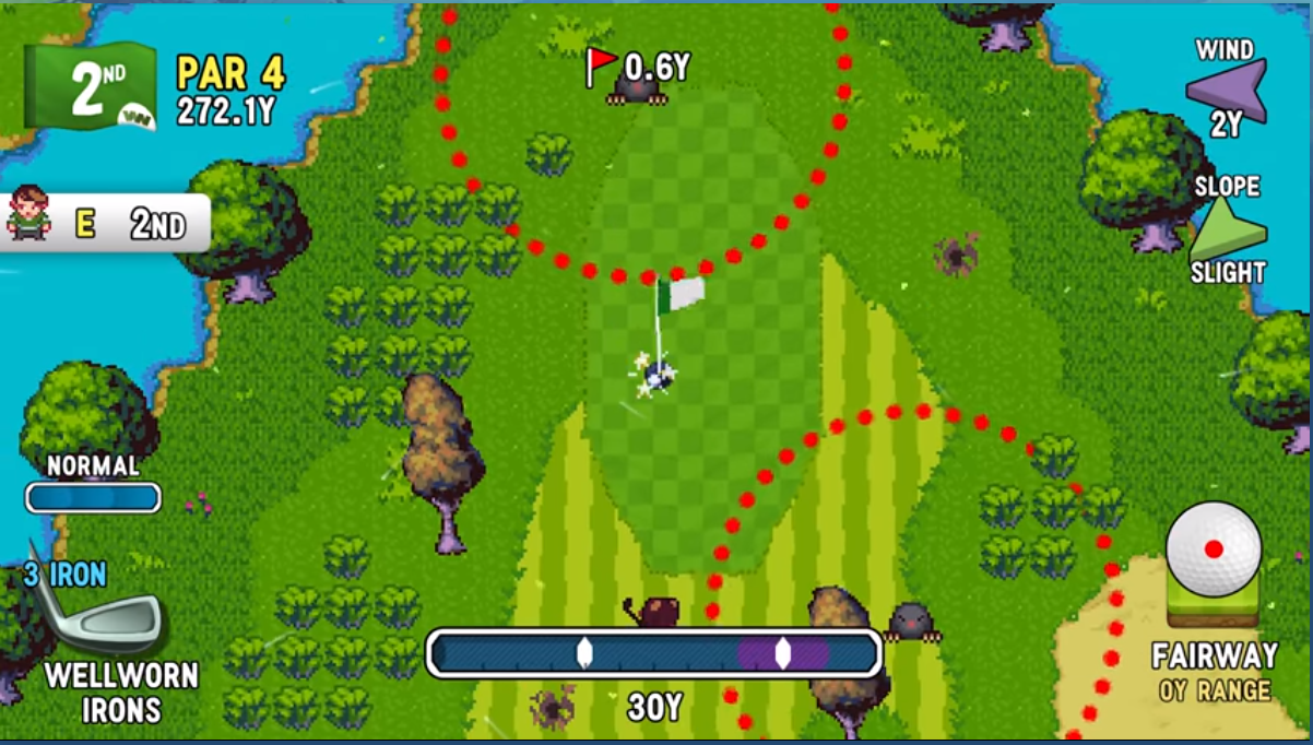
For increased precision or to introduce additional gameplay mechanics, it may be preferable in some cases to calculate a trajectory in 2D using two input sources. Typically, this takes the form of first determining the direction of the trajectory and then determining the 'strength' of the launch. Mathematically, this is equivalent to detrmining a unit vector \((x_0,y_0)\) of length one and then scaling it by a scalar 'strength' number \(s\). The final trajectory is then: $$(x,y) = (x_0,y_0) \times s = (sx_0,sy_0)$$ This is commonly seen in games like Golf Story (shown below), where the player first uses mouse/cursor movement to determine a direction unit vector \((x_0,y_0)\) and then interacts in some way with a 'strength' user interface (usually timing-based).

Source

Golf Story uses a power bar (bottom) to set the scalar shot strength \(s\)

Double Input (3D)

It is of course not possible to populate a trajectory vector in 3D space \((x,y,z)\) by using only mouse movement - there will be some trajectories that simply cannot be made, as even with predetermined \(x\) and \(y\) components there are an infinite number of trajectories as \(z\) varies. Hence, we must use at least two input sources. In my 3D golf prototype, I decided to use the mouse movement to determine the \(x\) and \(y\) components of the trajectory and the mouse wheel to determine the \(z\) component. This results in an intuitive and fast method of producing trajectories, whilst retaining a good level of precision.

Generating a Trajectory in 3D with Two Inputs

There is one aspect of this trajectory that could be remedied - keeping the endpoint of the trajectory stationary as the \(z\) component changes. As you can see in the demonstration below, as the player scrolls the mouse wheel (and consequently alters the \(z\) component) the endpoint of the trajectory moves significantly. This can make it difficult for the player to aim precisely. The next section details an efficient method to tackle this problem and keep the endpoint of the trajectory stationary.

Keeping the Endpoint of a Trajectory stationary

This section will detail the method that I devised to stabilise the endpoint of a trajectory as one of the vector components varies - the result in-game can be seen in the demonstration below. Note that as the heigh of the trajectory is changed by the player (the \(z\) component of the trajectory), the red endpoint of the trajectory remains stationary. This allows the player to have a lot more control and precision.

Keeping the Endpoint of a Trajectory Stationary in 3D Space

Problem Definition

Mathematically, the player is only changing the \(z\) component of the trajectory. Hence, given an initial trajectory \((x,y,z)\), we want to find a trajectory \((\overline{x},\overline{y},\overline{z})\) such that the endpoint of the trajectories are the same. Note also that \(x,y,z,\overline{z}\) are all known quantities since we know the original trajectory \((x,y,z)\) and we know the new height generated by the player \(\overline{z}\). It remains to find only \(\overline{x}\) and \(\overline{y}\).

Another observation that further simplifies this problem mathematically is that we must have both $$\overline{x} = \alpha x$$ $$\overline{y} = \alpha y$$ where \(\alpha\) is a scalar constant. To see this intuitively, observe that the components \(x\) and \(y\) of a trajectory provide the 'direction' of launch and the \(z\) component the 'height'. If this relationship was not true, then the direction of the two trajectories would be different and the endpoints could never be the same. This will not be proved mathematically here, although an illustration is provided below.

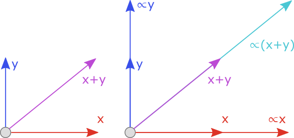Scaling a trajectory by a scalar

Whilst the mathematical proof is somewhat complicated, it turns out that the solution is surprisingly simple: $$\alpha = \frac{z}{\overline{z}}$$ and so we can simply scale our \(x\) and \(y\) component by this factor as described previously to obtain our new trajectory: $$(\overline{x},\overline{y},\overline{z}) = \left(\frac{z}{\overline{z}}x,\frac{z}{\overline{z}}y,\overline{z}\right)$$ For details of the proof, and how I arrived at this conclusion, see the next few sections!

Determining the Endpoint Location

We need to make sure that both trajectories \((x,y,z)\) and (\overline{x},\overline{y},\overline{z})\) have the same endpoint. In other words, they need to travel the same distance along the line \(\alpha(x+y)\) as demonstrated earlier. We can reduce the problem to 2 dimensions by considering the trajectory in the plane parallel to the lines \(x+y\) and \(z\) as pictured below, where \(t\) is the initial trajectory.

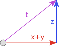Reducing the Problem to 2 Dimensions

We can now use the equations of motion (with constant acceleration) to calculate the total distance travelled \(s\) under the initial trajectory \((x,y,z)\): $$s = ut + \frac{1}{2}at^2$$ where $$u = \text{Initial Velocity}$$ $$t = \text{Time elapsed}$$ $$a = \text{Accelleration}$$ Since we have a number of unkown variables, we begin by considering movement only in the 'upwards' \(z\) direction. This will allow us to calculate the time that it takes for the projectile to hit the ground after launch. Here, we have that: $$u = z$$ $$a = -g$$ $$s = 0$$ where \(g\) is the gravitational constant (usually 9.8 in most game engines) and \(s=0\) because we want the time elapsed when the projectile is at distance 0 - it has returned to the ground plane. Solving this equation, where \(t \neq 0\), we obtain: $$0 = zt - \frac{1}{2}gt^2$$ $$\frac{1}{2}gt = z$$ $$t = \frac{2z}{g}$$ Now that we have the time it takes for the projectile to return to the ground plane, we can calculate the total distance travelled. Considering movement in the direction \(x+y\) now, we return to the equation \(s = ut + \frac{1}{2}at^2\) where: $$u = |x+y|$$ $$a = 0$$ $$t = \frac{2z}{g}$$ Note that we could have \(a=-l\) for some linear damping factor \(l\), which is a common inclusion in most game engines. However, this ends up having no bearing on the result and so is ommited here for simplicity. Solving this equation gives us the total distance travelled in the line \(x+y\) and hence the endpoint: $$s = \frac{2z|x+y|}{g}$$

Determining the scale factor \(\alpha\)

It remains to calculate the scale factor \(\alpha\). Using the equation derived previously, we have the distance travelled under the initial trajectory \(x,y,z\): $$s = \frac{2z|x+y|}{g}$$ and, following the same logic, the distance travelled under the new trajectory \((\overline{x},\overline{y},\overline{z})\): $$\overline{s} = \frac{2\overline{z}|\overline{x}+\overline{y}|}{g}$$ We want the endpoint to be the same, so we can equate these two identities: $$\frac{2z|x+y|}{g} = \frac{2\overline{z}|\overline{x}+\overline{y}|}{g}$$ $$z|x+y| = \overline{z}|\overline{x}+\overline{y}|$$ $$z\sqrt{x^2+y^2} = \overline{z}\sqrt{\overline{x}^2+\overline{y}^2}$$ $$z^2(x^2+y^2) = \overline{z}^2(\overline{x}^2+\overline{y}^2)$$ $$\overline{x}^2+\overline{y}^2 = \frac{z^2}{\overline{z}^2}(x^2+y^2)$$ Recall that \(x,y,z\) and \(\overline{z}\) are all know quantities. Now, using the fact that \(\overline{x}=\alpha x\) and \(\overline{y}=\alpha y\), we have: $$\alpha^2(x^2+y^2) = \frac{z^2}{\overline{z}^2}(x^2+y^2)$$ $$\alpha^2 = \frac{z^2}{\overline{z}^2}$$ and finally, as claimed earlier, we have our scale factor: $$\alpha = \frac{z}{\overline{z}}$$ and corresponding scaled trajectory with the same endpoint: $$(\overline{x},\overline{y},\overline{z}) = \left(\frac{z}{\overline{z}}x,\frac{z}{\overline{z}}y,\overline{z}\right)$$

The following code block demonstrates how this can be used to scale a trajectory whilst keeping a stationary end point. This function is called each time that the player tries to adjust the (z) component of the trajectory - it simply scales both the (x) and (y) components according to the mathematics above:

void APlayerBallController::scaleTrajectory(float oldZ, float newZ)
{
	float alpha = oldZ / newZ;
	currentX = currentX * alpha;
	currentY = currentY * alpha;
	return;
}

Return Home